bayesml.autoregressive package#
Module contents#
The linear autoregressive model with the normal-gamma prior distribution.
The stochastic data generative model is as follows:
\(d \in \mathbb{N}\): the degree of the model
\(n \in \mathbb{N}\): time index
\(x_n \in \mathbb{R}\): a data point at \(n\)
\(\boldsymbol{x}'_n := [1, x_{n-d}, x_{n-d+1}, \dots , x_{n-1}]^\top \in \mathbb{R}^{d+1}\). Here we assume \(x_n\) for \(n < 1\) is given as a initial value.
\(\boldsymbol{\theta} \in \mathbb{R}^{d+1}\): a regression coefficient parameter
\(\tau \in \mathbb{R}_{>0}\): a precision parameter of noise
The prior distribution is as follows:
\(\boldsymbol{\mu}_0 \in \mathbb{R}^{d+1}\): a hyperparameter for \(\boldsymbol{\theta}\)
\(\boldsymbol{\Lambda}_0 \in \mathbb{R}^{(d+1) \times (d+1)}\): a hyperparameter for \(\boldsymbol{\theta}\) (a positive definite matrix)
\(| \boldsymbol{\Lambda}_0 | \in \mathbb{R}\): the determinant of \(\boldsymbol{\Lambda}_0\)
\(\alpha_0 \in \mathbb{R}_{>0}\): a hyperparameter for \(\tau\)
\(\beta_0 \in \mathbb{R}_{>0}\): a hyperparameter for \(\tau\)
\(\Gamma(\cdot): \mathbb{R}_{>0} \to \mathbb{R}\): the Gamma function
The posterior distribution is as follows:
\(x^n := [x_1, x_2, \dots , x_n]^\top \in \mathbb{R}^n\): given data
\(\boldsymbol{X}_n = [\boldsymbol{x}'_1, \boldsymbol{x}'_2, \dots , \boldsymbol{x}'_n]^\top \in \mathbb{R}^{n \times (d+1)}\)
\(\boldsymbol{\mu}_n \in \mathbb{R}^{d+1}\): a hyperparameter for \(\boldsymbol{\theta}\)
\(\boldsymbol{\Lambda}_n \in \mathbb{R}^{(d+1) \times (d+1)}\): a hyperparameter for \(\boldsymbol{\theta}\) (a positive definite matrix)
\(\alpha_n \in \mathbb{R}_{>0}\): a hyperparameter for \(\tau\)
\(\beta_n \in \mathbb{R}_{>0}\): a hyperparameter for \(\tau\)
where the updating rules of the hyperparameters are
The predictive distribution is as follows:
\(x_{n+1} \in \mathbb{R}\): a new data point
\(m_\mathrm{p} \in \mathbb{R}\): a parameter
\(\lambda_\mathrm{p} \in \mathbb{R}_{>0}\): a parameter
\(\nu_\mathrm{p} \in \mathbb{R}_{>0}\): a parameter
where the parameters are obtained from the hyperparameters of the posterior distribution as follows.
- class bayesml.autoregressive.GenModel(c_degree, theta_vec=None, tau=1.0, h_mu_vec=None, h_lambda_mat=None, h_alpha=1.0, h_beta=1.0, seed=None)#
Bases:
GenerativeThe stochastic data generative model and the prior distribution.
- Parameters:
- c_degreeint
a positive integer.
- theta_vecnumpy ndarray, optional
a vector of real numbers, which includs the constant term, by default [0.0, 0.0, … , 0.0]
- taufloat, optional
a positive real number, by default 1.0
- h_mu_vecnumpy ndarray, optional
a vector of real numbers, by default [0.0, 0.0, … , 0.0]
- h_lambda_matnumpy ndarray, optional
a positive definate matrix, by default the identity matrix
- h_alphafloat, optional
a positive real number, by default 1.0
- h_betafloat, optional
a positive real number, by default 1.0
- seed{None, int}, optional
A seed to initialize numpy.random.default_rng(), by default None
Methods
Generate the parameter from the prior distribution.
gen_sample(sample_length[, initial_values])Generate a sample from the stochastic data generative model.
Get constants of GenModel.
Get the hyperparameters of the prior distribution.
Get the parameter of the sthocastic data generative model.
load_h_params(filename)Load the hyperparameters to h_params.
load_params(filename)Load the parameters saved by
save_params.save_h_params(filename)Save the hyperparameters using python
picklemodule.save_params(filename)Save the parameters using python
picklemodule.save_sample(filename, sample_length[, ...])Save the generated sample as NumPy
.npzformat.set_h_params([h_mu_vec, h_lambda_mat, ...])Set the hyperparameters of the prior distribution.
set_params([theta_vec, tau])Set the parameter of the sthocastic data generative model.
visualize_model([sample_length, sample_num, ...])Visualize the stochastic data generative model and generated samples.
- get_constants()#
Get constants of GenModel.
- Returns:
- constantsdict of {str: int}
"c_degree": the value ofself.c_degree
- set_h_params(h_mu_vec=None, h_lambda_mat=None, h_alpha=None, h_beta=None)#
Set the hyperparameters of the prior distribution.
- Parameters:
- h_mu_vecnumpy ndarray, optional
a vector of real numbers, by default None.
- h_lambda_matnumpy ndarray, optional
a positive definate matrix, by default None.
- h_alphafloat, optional
a positive real number, by default None.
- h_betafloat, optional
a positive real number, by default None.
- get_h_params()#
Get the hyperparameters of the prior distribution.
- Returns:
- h_paramsdict of {str: float or numpy ndarray}
"h_mu_vec": The value ofself.h_mu_vec"h_lambda_mat": The value ofself.h_lambda_mat"h_alpha": The value ofself.h_alpha"h_beta": The value ofself.h_beta
- gen_params()#
Generate the parameter from the prior distribution.
The generated vaule is set at
self.theta_vecand ``self.tau.
- set_params(theta_vec=None, tau=None)#
Set the parameter of the sthocastic data generative model.
- Parameters:
- theta_vecnumpy ndarray, optional
a vector of real numbers, by default None
- taufloat, optional, optional
a positive real number, by default None
- get_params()#
Get the parameter of the sthocastic data generative model.
- Returns:
- paramsdict of {str: float or numpy ndarray}
"theta_vec": The value ofself.theta_vec."tau": The value ofself.tau.
- gen_sample(sample_length, initial_values=None)#
Generate a sample from the stochastic data generative model.
- Parameters:
- sample_lengthint
A positive integer
- initial_valulesnumpy ndarray, optional
1 dimensional float array whose size coincide with
self.c_degree, by default None.
- Returns:
- xnumpy ndarray
1 dimensional float array whose size is
sammple_length.
- save_sample(filename, sample_length, initial_values=None)#
Save the generated sample as NumPy
.npzformat.It is saved as a NpzFile with keyword: “x”.
- Parameters:
- filenamestr
The filename to which the sample is saved.
.npzwill be appended if it isn’t there.- sample_lengthint
A positive integer
- initial_valulesnumpy ndarray, optional
1 dimensional float array whose size coincide with
self.c_degree, by default None.
See also
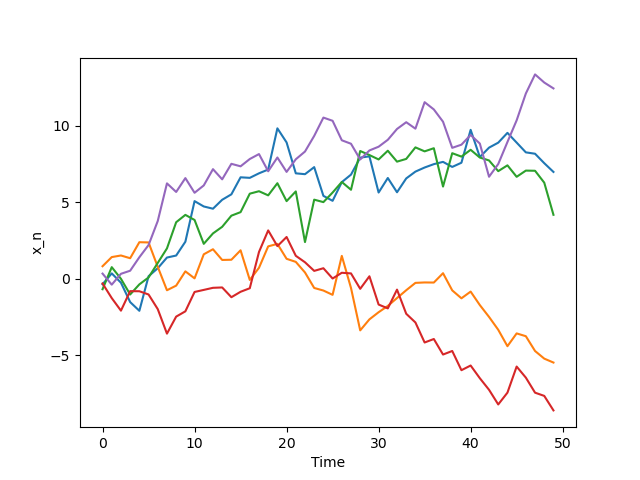
- visualize_model(sample_length=50, sample_num=5, initial_values=None)#
Visualize the stochastic data generative model and generated samples.
- Parameters:
- sample_lengthint, optional
A positive integer, by default 50
- sample_numint, optional
A positive integer, by default 5
- initial_valulesnumpy ndarray, optional
1 dimensional float array whose size coincide with
self.c_degree, by default None.
Examples
>>> import numpy as np
>>> from bayesml import autoregressive
>>> model = autoregressive.GenModel(c_degree=1,theta_vec=np.array([0,1]))
>>> model.visualize_model()
theta_vec:[0,1]
tau:1.0
- class bayesml.autoregressive.LearnModel(c_degree, h0_mu_vec=None, h0_lambda_mat=None, h0_alpha=1.0, h0_beta=1.0)#
Bases:
Posterior,PredictiveMixinThe posterior distribution and the predictive distribution.
- Parameters:
- c_degreeint
a positive integer.
- h0_mu_vecnumpy ndarray, optional
a vector of real numbers, by default [0.0, 0.0, … , 0.0]
- h0_lambda_matnumpy ndarray, optional
a positive definate matrix, by default the identity matrix
- h0_alphafloat, optional
a positive real number, by default 1.0
- h0_betafloat, optional
a positive real number, by default 1.0
- Attributes:
- hn_mu_vecnumpy ndarray
a vector of real numbers
- hn_lambda_matnumpy ndarray
a positive definate matrix
- hn_alphafloat
a positive real number
- hn_betafloat
a positive real number
- p_mfloat
a positive real number
- p_lambdafloat
a positive real number
- p_nufloat
a positive real number
Methods
Calculate the parameters of the predictive distribution.
estimate_params([loss])Estimate the parameter of the stochastic data generative model under the given criterion.
Get constants of LearnModel.
Get the initial values of the hyperparameters of the posterior distribution.
Get the hyperparameters of the posterior distribution.
Get the parameters of the predictive distribution.
load_h0_params(filename)Load the hyperparameters to h0_params.
load_hn_params(filename)Load the hyperparameters to hn_params.
make_prediction([loss])Predict a new data point under the given criterion.
overwrite_h0_params()Overwrite the initial values of the hyperparameters of the posterior distribution by the learned values.
pred_and_update(x[, loss])Predict a new data point and update the posterior sequentially.
predict_interval([credibility])Credible interval of the prediction.
reset_hn_params()Reset the hyperparameters of the posterior distribution to their initial values.
save_h0_params(filename)Save the hyperparameters using python
picklemodule.save_hn_params(filename)Save the hyperparameters using python
picklemodule.set_h0_params([h0_mu_vec, h0_lambda_mat, ...])Set initial values of the hyperparameter of the posterior distribution.
set_hn_params([hn_mu_vec, hn_lambda_mat, ...])Set updated values of the hyperparameter of the posterior distribution.
update_posterior(x[, padding])Update the hyperparameters of the posterior distribution using traning data.
Visualize the posterior distribution for the parameter.
- get_constants()#
Get constants of LearnModel.
- Returns:
- constantsdict of {str: int}
"c_degree": the value ofself.c_degree
- set_h0_params(h0_mu_vec=None, h0_lambda_mat=None, h0_alpha=None, h0_beta=None)#
Set initial values of the hyperparameter of the posterior distribution.
Note that the parameters of the predictive distribution are also calculated from
self.h0_mu_vec,slef.h0_lambda_mat,self.h0_alphaandself.h0_beta.- Parameters:
- h0_mu_vecnumpy ndarray, optional
a vector of real numbers, by default None.
- h0_lambda_matnumpy ndarray, optional
a positive definate matrix, by default None.
- h0_alphafloat, optional
a positive real number, by default None.
- h0_betafloat, optional
a positive real number, by default None.
- get_h0_params()#
Get the initial values of the hyperparameters of the posterior distribution.
- Returns:
- h0_paramsdict of {str: float or numpy ndarray}
"h0_mu_vec": The value ofself.h0_mu_vec"h0_lambda_mat": The value ofself.h0_lambda_mat"h0_alpha": The value ofself.h0_alpha"h0_beta": The value ofself.h0_beta
- get_hn_params()#
Get the hyperparameters of the posterior distribution.
- Returns:
- hn_paramsdict of {str: float or numpy ndarray}
"hn_mu_vec": The value ofself.hn_mu_vec"hn_lambda_mat": The value ofself.hn_lambda_mat"hn_alpha": The value ofself.hn_alpha"hn_beta": The value ofself.hn_beta
- set_hn_params(hn_mu_vec=None, hn_lambda_mat=None, hn_alpha=None, hn_beta=None)#
Set updated values of the hyperparameter of the posterior distribution.
Note that the parameters of the predictive distribution are also calculated from
self.hn_mu_vec,slef.hn_lambda_mat,self.hn_alphaandself.hn_beta.- Parameters:
- hn_mu_vecnumpy ndarray, optional
a vector of real numbers, by default None.
- hn_lambda_matnumpy ndarray, optional
a positive definate matrix, by default None.
- hn_alphafloat, optional
a positive real number, by default None.
- hn_betafloat, optional
a positive real number, by default None.
- update_posterior(x, padding=None)#
Update the hyperparameters of the posterior distribution using traning data.
- Parameters:
- xnumpy ndarray
1 dimensional float array
- paddingstr, optional
Padding option for data values at negative time points. Default is
None, in which case the firstself.c_degreevalues ofXare used as initial values. If “zeros” is given, the zero vector is used as a initial value.
- estimate_params(loss='squared')#
Estimate the parameter of the stochastic data generative model under the given criterion.
Note that the criterion is applied to estimating
theta_vecandtauindependently. Therefore, a tuple of the student’s t-distribution and the gamma distribution will be returned when loss=”KL”- Parameters:
- lossstr, optional
Loss function underlying the Bayes risk function, by default “squared”. This function supports “squared”, “0-1”, “abs”, and “KL”.
- Returns:
- Estimatestuple of {numpy ndarray, float, None, or rv_frozen}
theta_vec_hat: the estimate for theta_vectau_hat: the estimate for tau
The estimated values under the given loss function. If it is not exist, None will be returned. If the loss function is “KL”, the posterior distribution itself will be returned as rv_frozen object of scipy.stats.
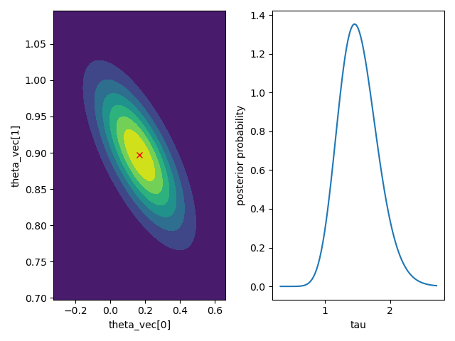
- visualize_posterior()#
Visualize the posterior distribution for the parameter.
Examples
>>> from bayesml import autoregressive
>>> gen_model = autoregressive.GenModel(c_degree=1,theta_vec=np.array([0,1]),tau=1.0)
>>> x = gen_model.gen_sample(50)
>>> learn_model = autoregressive.LearnModel()
>>> learn_model.update_posterior(x)
>>> learn_model.visualize_posterior()
- get_p_params()#
Get the parameters of the predictive distribution.
- Returns:
- p_paramsdict of {str: float}
"p_m": The value ofself.p_m"p_lambda": The value ofself.p_lambda"p_nu": The value ofself.p_nu
- calc_pred_dist(x)#
Calculate the parameters of the predictive distribution.
- Parameters:
- xnumpy ndarray
1 dimensional float array whose size is
self.c_degree
- make_prediction(loss='squared')#
Predict a new data point under the given criterion.
- Parameters:
- lossstr, optional
Loss function underlying the Bayes risk function, by default “squared”. This function supports “squared”, “0-1”, “abs”, and “KL”.
- Returns:
- Predicted_value{float, rv_frozen}
The predicted value under the given loss function. If the loss function is “KL”, the predictive distribution itself will be returned as rv_frozen object of scipy.stats.
- predict_interval(credibility=0.95)#
Credible interval of the prediction.
- Parameters:
- credibilityfloat, optional
A posterior probability that the interval conitans the paramter, by default 0.95
- Returns:
- lower, upper: float
The lower and the upper bound of the interval
- pred_and_update(x, loss='squared')#
Predict a new data point and update the posterior sequentially.
- Parameters:
- xnumpy ndarray
1 dimensional float array whose size is
self.c_degree + 1, which consists of theself.c_degreenumber of past values and the current value.- lossstr, optional
Loss function underlying the Bayes risk function, by default “squared”. This function supports “squared”, “0-1”, “abs”, and “KL”.
- Returns:
- Predicted_value{float, rv_frozen}
The predicted value under the given loss function. If the loss function is “KL”, the predictive distribution itself will be returned as rv_frozen object of scipy.stats.