bayesml.metatree package

bayesml.metatree package#

Module contents#

The stochastic data generative model is as follows:

\(\boldsymbol{x}=[x_1, \ldots, x_p, x_{p+1}, \ldots , x_{p+q}]\) : an explanatory variable. The first \(p\) variables are continuous. The other \(q\) variables are categorical.
\(\mathcal{Y}\) : a space of an objective variable
\(y \in \mathcal{Y}\) : an objective variable
\(D_\mathrm{max} \in \mathbb{N}\) : the maximum depth of trees
\(T\) : a tree whose depth is smaller than or equal to \(D_\mathrm{max}\)
\(\mathcal{T}\) : a set of \(T\)
\(s\) : a node of a tree
\(\mathcal{S}\) : a set of \(s\)
\(\mathcal{I}(T)\) : a set of inner nodes of \(T\)
\(\mathcal{L}(T)\) : a set of leaf nodes of \(T\)
\(\boldsymbol{k}=(k_s)_{s \in \mathcal{S}}\) : feature assignment vector where \(k_s \in \{1, 2,\ldots,p+q\}\). If \(k_s \leq p\), the node \(s\) has a threshold.
\(\boldsymbol{\theta}=(\theta_s)_{s \in \mathcal{S}}\) : a set of parameter
\(s(\boldsymbol{x}) \in \mathcal{L}(T)\) : a leaf node of \(T\) corresponding to \(\boldsymbol{x}\), which is determined according to \(\boldsymbol{k}\) and the thresholds.

\[p(y | \boldsymbol{x}, \boldsymbol{\theta}, T, \boldsymbol{k})=p(y | \theta_{s(\boldsymbol{x})})\]

The prior distribution is as follows:

\(g_{0,s} \in [0,1]\) : a hyperparameter assigned to \(s \in \mathcal{S}\)
\(M_{T, \boldsymbol{k}}\) : a meta-tree for \((T, \boldsymbol{k})\)
\(\mathcal{T}_{M_{T, \boldsymbol{k}}}\) : a set of \(T\) represented by a meta-tree \(M_{T, \boldsymbol{k}}\)
\(B \in \mathbb{N}\) : the number of meta-trees
\(\mathcal{M}=\{(T_1, \boldsymbol{k}_1), (T_2, \boldsymbol{k}_2), \ldots, (T_B, \boldsymbol{k}_B) \}\) for \(B\) meta-trees \(M_{T_1, \boldsymbol{k}_1}, M_{T_2, \boldsymbol{k}_2}, \dots, M_{T_B, \boldsymbol{k}_B}\). (These meta-trees must be given beforehand by some method, e.g., constructed from bootstrap samples similar to the random forest.)

For \(T' \in M_{T, \boldsymbol{k}}\),

\[p(T')=\prod_{s \in \mathcal{I}(T')} g_{0,s} \prod_{s' \in \mathcal{L}(T')} (1-g_{0,s'}),\]

where \(g_{0,s}=0\) for a leaf node \(s\) of a meta-tree \(M_{T, \boldsymbol{k}}\).

For \(\boldsymbol{k}_b \in \{\boldsymbol{k}_1, \boldsymbol{k}_2, \ldots, \boldsymbol{k}_B \}\),

\[p(\boldsymbol{k}_b) = \frac{1}{B}.\]

The posterior distribution is as follows:

\(n \in \mathbb{N}\) : a sample size
\(\boldsymbol{x}^n = \{ \boldsymbol{x}_1, \boldsymbol{x}_2, \ldots, \boldsymbol{x}_n \}\)
\(y^n = \{ y_1, y_2, \ldots, y_n \}\)
\(g_{n,s} \in [0,1]\) : a hyperparameter

For \(T' \in M_{T, \boldsymbol{k}}\),

\[p(T' | \boldsymbol{x}^n, y^n, \boldsymbol{k})=\prod_{s \in \mathcal{I}(T')} g_{n,s} \prod_{s' \in \mathcal{L}(T')} (1-g_{n,s'}),\]

where the updating rules of the hyperparameter are as follows.

\[\begin{split}g_{i,s} = \begin{cases} g_{0,s} & (i = 0),\\ \frac{g_{i-1,s} \tilde{q}_{s_{\mathrm{child}}}(y_i | \boldsymbol{x}_i, \boldsymbol{x}^{i-1}, y^{i-1}, M_{T, \boldsymbol{k}})}{\tilde{q}_s(y_i | \boldsymbol{x}_i, \boldsymbol{x}^{i-1}, y^{i-1}, M_{T, \boldsymbol{k}})} &(\mathrm{otherwise}), \end{cases}\end{split}\]

where \(s_{\mathrm{child}}\) is the child node of \(s\) on the path corresponding to \(\boldsymbol{x}_{i}\) in \(M_{T, \boldsymbol{k}}\) and

\[\begin{split}&\tilde{q}_s(y_{i} | \boldsymbol{x}_{i}, \boldsymbol{x}^{i-1}, y^{i-1}, M_{T, \boldsymbol{k}}) \\ &= \begin{cases} q_s(y_{i} | \boldsymbol{x}_{i}, \boldsymbol{x}^{i-1}, y^{i-1}, \boldsymbol{k}),& (s \ {\rm is \ the \ leaf \ node \ of} \ M_{T, \boldsymbol{k}}),\\ (1-g_{i-1,s}) q_s(y_{i} | \boldsymbol{x}_{i}, \boldsymbol{x}^{i-1}, y^{i-1}, \boldsymbol{k}) \\ \qquad + g_{i-1,s} \tilde{q}_{s_{\mathrm{child}}}(y_{i} | \boldsymbol{x}_{i}, \boldsymbol{x}^{i-1}, y^{i-1}, M_{T, \boldsymbol{k}}),& ({\rm otherwise}), \end{cases}\end{split}\]

\[q_s(y_{i} | \boldsymbol{x}_{i}, \boldsymbol{x}^{i-1}, y^{i-1}, \boldsymbol{k})=\int p(y_i | \boldsymbol{x}_i, \boldsymbol{\theta}, T, \boldsymbol{k}) p(\boldsymbol{\theta} | \boldsymbol{x}^{i-1}, y^{i-1}, T, \boldsymbol{k}) \mathrm{d} \boldsymbol{\theta}, \quad s \in \mathcal{L}(T)\]

For \(\boldsymbol{k}_b \in \{\boldsymbol{k}_1, \boldsymbol{k}_2, \ldots, \boldsymbol{k}_B \}\),

\[p(\boldsymbol{k}_b | \boldsymbol{x}^n, y^n)\propto \prod_{i=1}^n \tilde{q}_{s_{\lambda}}(y_{i}|\boldsymbol{x}_{i},\boldsymbol{x}^{i-1}, y^{i-1}, M_{T_b, \boldsymbol{k}_b}),\]

where \(s_{\lambda}\) is the root node of \(M_{T_b, \boldsymbol{k}_b}\).

The predictive distribution is as follows:

\[p(y_{n+1}| \boldsymbol{x}_{n+1}, \boldsymbol{x}^n, y^n) = \sum_{b = 1}^B p(\boldsymbol{k}_b | \boldsymbol{x}^n, y^n) \tilde{q}_{s_{\lambda}}(y_{n+1}|\boldsymbol{x}_{n+1},\boldsymbol{x}^n, y^n, M_{T_b, \boldsymbol{k}_b})\]

The expectation of the predictive distribution can be calculated as follows.

\[\mathbb{E}_{p(y_{n+1}| \boldsymbol{x}_{n+1}, \boldsymbol{x}^n, y^n)} [Y_{n+1}| \boldsymbol{x}_{n+1}, \boldsymbol{x}^n, y^n] = \sum_{b = 1}^B p(\boldsymbol{k}_b | \boldsymbol{x}^n, y^n) \mathbb{E}_{\tilde{q}_{s_{\lambda}}(y_{n+1}|\boldsymbol{x}_{n+1},\boldsymbol{x}^n, y^n, M_{T_b, \boldsymbol{k}_b})} [Y_{n+1}| \boldsymbol{x}_{n+1}, \boldsymbol{x}^n, y^n, \boldsymbol{k}_b],\]

where the expectation for \(\tilde{q}\) is recursively given as follows.

\[\begin{split}&\mathbb{E}_{\tilde{q}_s(y_{n+1} | \boldsymbol{x}_{n+1}, \boldsymbol{x}^n, y^n, M_{T_b, \boldsymbol{k}_b})} [Y_{n+1} | \boldsymbol{x}_{n+1}, \boldsymbol{x}^n, y^n, \boldsymbol{k}_b] \\ &= \begin{cases} \mathbb{E}_{q_s(y_{n+1} | \boldsymbol{x}_{n+1}, \boldsymbol{x}^n, y^n, \boldsymbol{k}_b)} [Y_{n+1} | \boldsymbol{x}_{n+1}, \boldsymbol{x}^n, y^n, \boldsymbol{k}_b],& (s \ {\rm is \ the \ leaf \ node \ of} \ M_{T_b, \boldsymbol{k}_b}),\\ (1-g_{n,s}) \mathbb{E}_{q_s(y_{n+1} | \boldsymbol{x}_{n+1}, \boldsymbol{x}^n, y^n, \boldsymbol{k}_b)} [Y_{n+1} | \boldsymbol{x}_{n+1}, \boldsymbol{x}^n, y^n, \boldsymbol{k}_b] \\ \qquad + g_{n,s} \mathbb{E}_{\tilde{q}_{s_{\mathrm{child}}}(y_{n+1} | \boldsymbol{x}_{n+1}, \boldsymbol{x}^n, y^n, M_{T_b, \boldsymbol{k}_b})} [Y_{n+1} | \boldsymbol{x}_{n+1}, \boldsymbol{x}^n, y^n, \boldsymbol{k}_b] ,& ({\rm otherwise}). \end{cases}\end{split}\]

References

Dobashi, N.; Saito, S.; Nakahara, Y.; Matsushima, T. Meta-Tree Random Forest: Probabilistic Data-Generative Model and Bayes Optimal Prediction. Entropy 2021, 23, 768. https://doi.org/10.3390/e23060768
Nakahara, Y.; Saito, S.; Kamatsuka, A.; Matsushima, T. Probability Distribution on Full Rooted Trees. Entropy 2022, 24, 328. https://doi.org/10.3390/e24030328

class bayesml.metatree.GenModel(c_dim_continuous, c_dim_categorical, c_max_depth=2, c_num_children_vec=2, c_num_assignment_vec=None, c_ranges=None, SubModel=<module 'bayesml.bernoulli' from 'C:\\Users\\nakahara\\Documents\\GitHub\\BayesML\\bayesml\\bernoulli\\__init__.py'>, sub_constants={}, root=None, h_k_weight_vec=None, h_g=0.5, sub_h_params={}, h_metatree_list=[], h_metatree_prob_vec=None, seed=None)#

Bases: Generative

The stochastice data generative model and the prior distribution

Parameters:

c_dim_continuousint: A non-negative integer
c_dim_categoricalint: A non-negative integer
c_num_children_vecnumpy.ndarray, optional: A vector of positive integers whose length is c_dim_continuous+c_dim_categorical, by default [2,2,…,2]. The first c_dim_continuous elements represent the numbers of children of continuous features at inner nodes. The other c_dim_categorial elements represent those of categorical features. If a single integer is input, it will be broadcasted.
c_max_depthint, optional: A positive integer, by default 2
c_num_assignment_vecnumpy.ndarray, optional: A vector of positive integers whose length is c_dim_continuous+c_dim_categorical. The first c_dim_continuous elements represent the maximum assignment numbers of continuous features on a path. The other c_dim_categorial elements represent those of categorical features. If it has a negative element (e.g., -1), the corresponding feature will be assigned any number of times. By default [c_max_depth,…,c_max_depth,1,…,1].
c_rangesnumpy.ndarray, optional: A numpy.ndarray whose size is (c_dim_continuous,2). A threshold for the k-th continuous feature will be generated between c_ranges[k,0] and c_ranges[k,1]. By default, [[-3,3],[-3,3],…,[-3,3]].
SubModelclass, optional: bernoulli, categorical, poisson, normal, exponential, or linearregression, by default bernoulli
sub_constantsdict, optional: constants for self.SubModel.GenModel, by default {}
rootmetatree._Node, optional: A root node of a meta-tree, by default a tree consists of only one node.
h_k_weight_vecnumpy.ndarray, optional: A vector of positive real numbers whose length is c_dim_continuous+c_dim_categorical, by default [1,…,1].
h_gfloat, optional: A real number in \([0, 1]\), by default 0.5
sub_h_paramsdict, optional: h_params for self.SubModel.GenModel, by default {}
h_metatree_listlist of metatree._Node, optional: Root nodes of meta-trees, by default []
h_metatree_prob_vecnumpy.ndarray, optional: A vector of real numbers in \([0, 1]\) that represents prior distribution of h_metatree_list, by default uniform distribution Sum of its elements must be 1.0.
seed{None, int}, optional: A seed to initialize numpy.random.default_rng(), by default None

Attributes:

c_dim_features: int: c_dim_continuous + c_dim_categorical

Methods

`gen_params`([feature_fix, threshold_fix, ...])	Generate the parameter from the prior distribution.
`gen_sample`([sample_size, x_continuous, ...])	Generate a sample from the stochastic data generative model.
`get_constants`()	Get constants of GenModel.
`get_h_params`()	Get the hyperparameters of the prior distribution.
`get_params`()	Get the parameter of the sthocastic data generative model.
`load_h_params`(filename)	Load the hyperparameters to h_params.
`load_params`(filename)	Load the parameters saved by `save_params`.
`save_h_params`(filename)	Save the hyperparameters using python `pickle` module.
`save_params`(filename)	Save the parameters using python `pickle` module.
`save_sample`(filename, sample_size[, x])	Save the generated sample as NumPy `.npz` format.
`set_h_params`([h_k_weight_vec, h_g, ...])	Set the hyperparameters of the prior distribution.
`set_params`([root])	Set the parameter of the sthocastic data generative model.
`visualize_model`([filename, format, ...])	Visualize the stochastic data generative model and generated samples.

get_constants()#

Get constants of GenModel.

Returns:

constantsdict of {str: int, numpy.ndarray}

"c_dim_continuous" : the value of self.c_dim_continuous
"c_dim_categorical" : the value of self.c_dim_categorical
"c_num_children_vec" : the value of self.c_num_children_vec
"c_max_depth" : the value of self.c_max_depth
"c_num_assignment_vec" : the value of self.c_num_assignment_vec
"c_ranges" : the value of self.c_ranges

set_h_params(h_k_weight_vec=None, h_g=None, sub_h_params=None, h_metatree_list=None, h_metatree_prob_vec=None)#

Set the hyperparameters of the prior distribution.

Parameters:

h_k_weight_vecnumpy.ndarray, optional: A vector of positive real numbers whose length is c_dim_continuous+c_dim_categorical, by default None.
h_gfloat, optional: A real number in \([0, 1]\), by default None
sub_h_paramsdict, optional: h_params for self.SubModel.GenModel, by default None
h_metatree_listlist of metatree._Node, optional: Root nodes of meta-trees, by default None
h_metatree_prob_vecnumpy.ndarray, optional: A vector of real numbers in \([0, 1]\) that represents prior distribution of h_metatree_list, by default None. Sum of its elements must be 1.0.

get_h_params()#

Get the hyperparameters of the prior distribution.

Returns:

h_paramsdict of {str: float, list, dict, numpy.ndarray}

"h_k_weight_vec" : the value of self.h_k_weight_vec
"h_g" : the value of self.h_g
"sub_h_params" : the value of self.sub_h_params
"h_metatree_list" : the value of self.h_metatree_list
"h_metatree_prob_vec" : the value of self.h_metatree_prob_vec

gen_params(feature_fix=False, threshold_fix=False, tree_fix=False, threshold_type='even')#

Generate the parameter from the prior distribution.

The generated vaule is set at self.root.

Parameters:

feature_fixbool, optional: If True, feature assignment indices will be fixed, by default False.
threshold_fixbool, optional: If True, thresholds for continuous features will be fixed, by default False. If feature_fix is False, threshold_fix must be False.
tree_fixbool, optional: If True, tree shape will be fixed, by default False. If feature_fix is False, tree_fix must be False.
threshold_type{‘even’, ‘random’}, optional: A type of threshold generating procedure, by default 'even' If 'even', self.c_ranges will be recursively divided by equal intervals. if 'random', self.c_ranges will be recursively divided by at random intervals.

set_params(root=None)#

Set the parameter of the sthocastic data generative model.

Parameters:

rootmetatree._Node, optional: A root node of a meta-tree, by default None.

get_params()#

Get the parameter of the sthocastic data generative model.

Returns:

paramsdict of {str:metatree._Node}

"root" : The value of self.root.

gen_sample(sample_size=None, x_continuous=None, x_categorical=None)#

Generate a sample from the stochastic data generative model.

Parameters:

sample_sizeint, optional: A positive integer, by default None
x_continuousnumpy ndarray, optional: 2 dimensional float array whose size is (sample_size,c_dim_continuous), by default None.
x_categoricalnumpy ndarray, optional: 2 dimensional int array whose size is (sample_size,c_dim_categorical), by default None. Each element x_categorical[i,j] must satisfy 0 <= x_categorical[i,j] < self.c_num_children_vec[self.c_dim_continuous+i].

Returns:

x_continuousnumpy ndarray: 2 dimensional float array whose size is (sample_size,c_dim_continuous).
x_categoricalnumpy ndarray, optional: 2 dimensional int array whose size is (sample_size,c_dim_categorical). Each element x_categorical[i,j] must satisfies 0 <= x_categorical[i,j] < self.c_num_children_vec[self.c_dim_continuous+i].
ynumpy ndarray: 1 dimensional array whose size is sample_size.

save_sample(filename, sample_size, x=None)#

Save the generated sample as NumPy .npz format.

It is saved as a NpzFile with keyword: “x”.

Parameters:

filenamestr: The filename to which the sample is saved. .npz will be appended if it isn’t there.
sample_sizeint, optional: A positive integer, by default None
x_continuousnumpy ndarray, optional: 2 dimensional float array whose size is (sample_size,c_dim_continuous), by default None.
x_categoricalnumpy ndarray, optional: 2 dimensional int array whose size is (sample_size,c_dim_categorical), by default None. Each element x_categorical[i,j] must satisfy 0 <= x_categorical[i,j] < self.c_num_children_vec[self.c_dim_continuous+i].

See also

numpy.savez_compressed

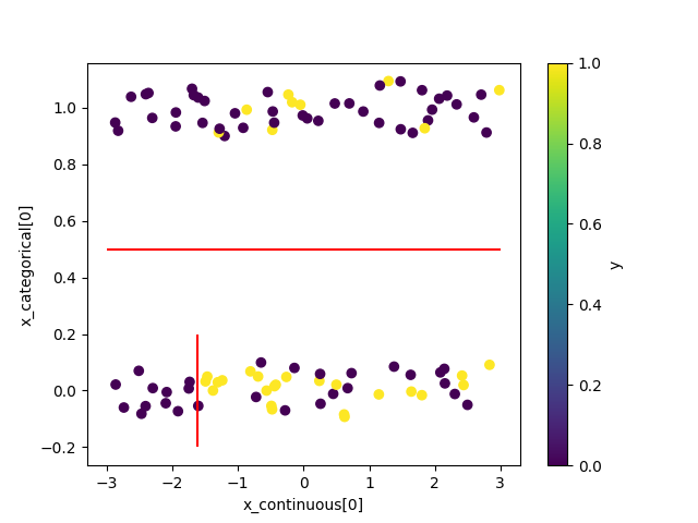
visualize_model(filename=None, format=None, sample_size=100, x_continuous=None, x_categorical=None)#

Visualize the stochastic data generative model and generated samples.

Note that values of categorical features will be shown with jitters.

Parameters:

filenamestr, optional: Filename for saving the figure, by default None
formatstr, optional: Rendering output format ("pdf", "png", …).
sample_sizeint, optional: A positive integer, by default 100
x_continuousnumpy ndarray, optional: 2 dimensional float array whose size is (sample_size,c_dim_continuous), by default None.
x_categoricalnumpy ndarray, optional: 2 dimensional int array whose size is (sample_size,c_dim_categorical), by default None. Each element x_categorical[i,j] must satisfy 0 <= x_categorical[i,j] < self.c_num_children_vec[self.c_dim_continuous+i].

See also

graphviz.Digraph

Examples

>>> from bayesml import metatree
>>> model = metatree.GenModel(
>>>     c_dim_continuous=1,
>>>     c_dim_categorical=1)
>>> model.gen_params(threshold_type='random')
>>> model.visualize_model()

class bayesml.metatree.LearnModel(c_dim_continuous, c_dim_categorical, c_num_children_vec=2, c_max_depth=2, c_num_assignment_vec=None, c_ranges=None, SubModel=<module 'bayesml.bernoulli' from 'C:\\Users\\nakahara\\Documents\\GitHub\\BayesML\\bayesml\\bernoulli\\__init__.py'>, sub_constants={}, h0_k_weight_vec=None, h0_g=0.5, sub_h0_params={}, h0_metatree_list=[], h0_metatree_prob_vec=None)#

Bases: Posterior, PredictiveMixin

The posterior distribution and the predictive distribution.

Parameters:

c_dim_continuousint: A non-negative integer
c_dim_categoricalint: A non-negative integer
c_num_children_vecnumpy.ndarray, optional: A vector of positive integers whose length is c_dim_continuous+c_dim_categorical, by default [2,2,…,2]. The first c_dim_continuous elements represent the numbers of children of continuous features at inner nodes. The other c_dim_categorial elements represent those of categorical features. If a single integer is input, it will be broadcasted.
c_max_depthint, optional: A positive integer, by default 2
c_num_assignment_vecnumpy.ndarray, optional: A vector of positive integers whose length is c_dim_continuous+c_dim_categorical. The first c_dim_continuous elements represent the maximum assignment numbers of continuous features on a path. The other c_dim_categorial elements represent those of categorical features. If it has a negative element (e.g., -1), the corresponding feature will be assigned any number of times. By default [c_max_depth,…,c_max_depth,1,…,1].
c_rangesnumpy.ndarray, optional: A numpy.ndarray whose size is (c_dim_continuous,2). A threshold for the k-th continuous feature will be generated between c_ranges[k,0] and c_ranges[k,1]. By default, [[-3,3],[-3,3],…,[-3,3]].
SubModelclass, optional: bernoulli, categorical, poisson, normal, exponential, or linearregression, by default bernoulli
sub_constantsdict, optional: constants for self.SubModel.LearnModel, by default {}
h0_k_weight_vecnumpy.ndarray, optional: A vector of positive real numbers whose length is c_dim_continuous+c_dim_categorical, by default [1,…,1].
h0_gfloat, optional: A real number in \([0, 1]\), by default 0.5
sub_h0_paramsdict, optional: h0_params for self.SubModel.LearnModel, by default {}
h0_metatree_listlist of metatree._Node, optional: Root nodes of meta-trees, by default []
h0_metatree_prob_vecnumpy.ndarray, optional: A vector of real numbers in \([0, 1]\) that represents prior distribution of h0_metatree_list, by default uniform distribution Sum of its elements must be 1.0.

Attributes:

c_dim_features: int: c_dim_continuous + c_dim_categorical
hn_k_weight_vecnumpy.ndarray: A vector of positive real numbers whose length is c_dim_continuous+c_dim_categorical
hn_gfloat: A real number in \([0, 1]\)
sub_hn_paramsdict: hn_params for self.SubModel.LearnModel
hn_metatree_listlist of metatree._Node: Root nodes of meta-trees
hn_metatree_prob_vecnumpy.ndarray: A vector of real numbers in \([0, 1]\) that represents prior distribution of h0_metatree_list. Sum of its elements is 1.0.

Methods

`calc_pred_dist`([x_continuous, x_categorical])	Calculate the parameters of the predictive distribution.
`estimate_params`([loss, visualize, filename, ...])	Estimate the parameter under the given criterion.
`get_constants`()	Get constants of LearnModel.
`get_h0_params`()	Get the hyperparameters of the prior distribution.
`get_hn_params`()	Get the hyperparameters of the posterior distribution.
`get_p_params`()	Get the parameters of the predictive distribution.
`load_h0_params`(filename)	Load the hyperparameters to h0_params.
`load_hn_params`(filename)	Load the hyperparameters to hn_params.
`make_prediction`([loss])	Predict a new data point under the given criterion.
`overwrite_h0_params`()	Overwrite the initial values of the hyperparameters of the posterior distribution by the learned values.
`pred_and_update`([x_continuous, ...])	Predict a new data point and update the posterior sequentially.
`reset_hn_params`()	Reset the hyperparameters of the posterior distribution to their initial values.
`save_h0_params`(filename)	Save the hyperparameters using python `pickle` module.
`save_hn_params`(filename)	Save the hyperparameters using python `pickle` module.
`set_h0_params`([h0_k_weight_vec, h0_g, ...])	Set the hyperparameters of the prior distribution.
`set_hn_params`([hn_k_weight_vec, hn_g, ...])	Set the hyperparameters of the posterior distribution.
`update_posterior`([x_continuous, ...])	Update the hyperparameters of the posterior distribution using traning data.
`visualize_posterior`([filename, format, ...])	Visualize the posterior distribution for the parameter.

get_constants()#

Get constants of LearnModel.

Returns:

constantsdict of {str: int, numpy.ndarray}

"c_dim_continuous" : the value of self.c_dim_continuous
"c_dim_categorical" : the value of self.c_dim_categorical
"c_num_children_vec" : the value of self.c_num_children_vec
"c_max_depth" : the value of self.c_max_depth
"c_num_assignment_vec" : the value of self.c_num_assignment_vec
"c_ranges" : the value of self.c_ranges

set_h0_params(h0_k_weight_vec=None, h0_g=None, sub_h0_params=None, h0_metatree_list=None, h0_metatree_prob_vec=None)#

Set the hyperparameters of the prior distribution.

Parameters:

h0_k_weight_vecnumpy.ndarray, optional: A vector of positive real numbers whose length is c_dim_continuous+c_dim_categorical, by default None.
h0_gfloat, optional: A real number in \([0, 1]\), by default None
sub_h0_paramsdict, optional: h0_params for self.SubModel.LearnModel, by default None
h0_metatree_listlist of metatree._Node, optional: Root nodes of meta-trees, by default None
h0_metatree_prob_vecnumpy.ndarray, optional: A vector of real numbers in \([0, 1]\) that represents prior distribution of h0_metatree_list, by default None. Sum of its elements must be 1.0.

get_h0_params()#

Get the hyperparameters of the prior distribution.

Returns:

h0_paramsdict of {str: float, list, dict, numpy.ndarray}

"h0_k_weight_vec" : the value of self.h0_k_weight_vec
"h0_g" : the value of self.h0_g
"sub_h0_params" : the value of self.sub_h0_params
"h0_metatree_list" : the value of self.h0_metatree_list
"h0_metatree_prob_vec" : the value of self.h0_metatree_prob_vec

set_hn_params(hn_k_weight_vec=None, hn_g=None, sub_hn_params=None, hn_metatree_list=None, hn_metatree_prob_vec=None)#

Set the hyperparameters of the posterior distribution.

Parameters:

hn_k_weight_vecnumpy.ndarray, optional: A vector of positive real numbers whose length is c_dim_continuous+c_dim_categorical, by default None.
hn_gfloat, optional: A real number in \([0, 1]\), by default None
sub_hn_paramsdict, optional: hn_params for self.SubModel.LearnModel, by default None
hn_metatree_listlist of metatree._Node, optional: Root nodes of meta-trees, by default None
hn_metatree_prob_vecnumpy.ndarray, optional: A vector of real numbers in \([0, 1]\) that represents prior distribution of hn_metatree_list, by default None. Sum of its elements must be 1.0.

get_hn_params()#

Get the hyperparameters of the posterior distribution.

Returns:

hn_paramsdict of {str: float, list, dict, numpy.ndarray}

"hn_k_weight_vec" : the value of self.hn_k_weight_vec
"hn_g" : the value of self.hn_g
"sub_hn_params" : the value of self.sub_hn_params
"hn_metatree_list" : the value of self.hn_metatree_list
"hn_metatree_prob_vec" : the value of self.hn_metatree_prob_vec

update_posterior(x_continuous=None, x_categorical=None, y=None, alg_type='MTRF', **kwargs)#

Update the hyperparameters of the posterior distribution using traning data.

Parameters:

x_continuousnumpy ndarray, optional: 2 dimensional float array whose size is (sample_size,c_dim_continuous), by default None.
x_categoricalnumpy ndarray, optional: 2 dimensional int array whose size is (sample_size,c_dim_categorical), by default None. Each element x_categorical[i,j] must satisfy 0 <= x_categorical[i,j] < self.c_num_children_vec[self.c_dim_continuous+i].
ynumpy ndarray: values of objective variable whose dtype may be int or float
alg_type{‘MTRF’, ‘given_MT’}, optional: type of algorithm, by default ‘MTRF’
**kwargsdict, optional: optional parameters of algorithms, by default {}

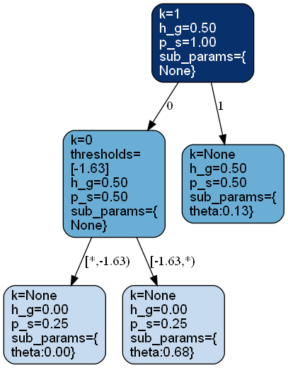
estimate_params(loss='0-1', visualize=True, filename=None, format=None)#

Estimate the parameter under the given criterion.

The approximate MAP meta-tree \(M_{T,\boldsymbol{k}_b} = \mathrm{argmax} p(M_{T,\boldsymbol{k}_{b'}} | \boldsymbol{x}^n, y^n)\) will be returned.

Parameters:

lossstr, optional: Loss function underlying the Bayes risk function, by default "0-1". This function supports only "0-1".
visualizebool, optional: If True, the estimated metatree will be visualized, by default True. This visualization requires graphviz.
filenamestr, optional: Filename for saving the figure, by default None
formatstr, optional: Rendering output format ("pdf", "png", …).

Returns:

map_rootmetatree._Node: The root node of the estimated meta-tree that also contains the estimated parameters in each node.

Warning

Multiple metatrees can represent equivalent model classes. This function does not take such duplication into account.

See also

graphviz.Digraph

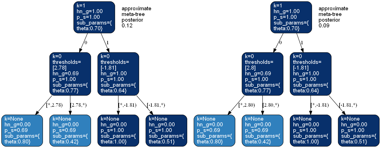
visualize_posterior(filename=None, format=None, num_metatrees=3, h_params=False)#

Visualize the posterior distribution for the parameter.

This method requires graphviz.

Parameters:

filenamestr, optional: Filename for saving the figure, by default None
formatstr, optional: Rendering output format ("pdf", "png", …).
num_metatreesint, optional: Number of metatrees to be visualized, by default 3.
h_paramsbool, optional: If True, hyperparameters at each node will be visualized. if False, estimated parameters at each node will be visulaized.

See also

graphviz.Digraph

Examples

>>> from bayesml import metatree
>>> gen_model = metatree.GenModel(
>>>     c_dim_continuous=1,
>>>     c_dim_categorical=1)
>>> gen_model.gen_params(threshold_type='random')
>>> x_continuous,x_categorical,y = gen_model.gen_sample(200)
>>> learn_model = metatree.LearnModel(
>>>     c_dim_continuous=1,
>>>     c_dim_categorical=1)
>>> learn_model.update_posterior(x_continuous,x_categorical,y)
>>> learn_model.visualize_posterior(num_metatrees=2)

get_p_params()#

Get the parameters of the predictive distribution.

This model does not have a simple parametric expression of the predictive distribution. Therefore, this function returns None.

Returns:

None

calc_pred_dist(x_continuous=None, x_categorical=None)#

Calculate the parameters of the predictive distribution.

Parameters:

x_continuousnumpy ndarray, optional: A float vector whose length is self.c_dim_continuous, by default None.
x_categoricalnumpy ndarray, optional: A int vector whose length is self.c_dim_categorical, by default None. Each element x_categorical[i] must satisfy 0 <= x_categorical[i] < self.c_num_children_vec[self.c_dim_continuous+i].

make_prediction(loss='squared')#

Predict a new data point under the given criterion.

Parameters:

lossstr, optional: Loss function underlying the Bayes risk function, by default “squared”. This function supports “squared”, “0-1”, and “KL”.

Returns:

predicted_value{float, numpy.ndarray}: The predicted value under the given loss function.

pred_and_update(x_continuous=None, x_categorical=None, y=None, loss='squared')#

Predict a new data point and update the posterior sequentially.

Parameters:

x_continuousnumpy ndarray, optional: A float vector whose length is self.c_dim_continuous, by default None.
x_categoricalnumpy ndarray, optional: A int vector whose length is self.c_dim_categorical, by default None. Each element x_categorical[i] must satisfy 0 <= x_categorical[i] < self.c_num_children_vec[self.c_dim_continuous+i].
ynumpy ndarray: values of objective variable whose dtype may be int or float
lossstr, optional: Loss function underlying the Bayes risk function, by default “squared”. This function supports “squared”, “0-1”, and “KL”.

Returns:

predicted_value{float, numpy.ndarray}: The predicted value under the given loss function.

bayesml.metatree package

Contents

bayesml.metatree package#

Module contents#