bayesml.categorical package#
Module contents#
The categorical distribution with the dirichlet prior distribution
The stochastic data generative model is as follows:
\(d\in \mathbb{Z}\): a dimension (\(d \geq 2\))
\(\boldsymbol{x} \in \{ 0, 1\}^d\): a data point, (a one-hot vector, i.e., \(\sum_{k=1}^d x_k=1\))
\(\boldsymbol{\theta} \in [0, 1]^d\): a parameter, (\(\sum_{k=1}^d \theta_k=1\))
The prior distribution is as follows:
\(\boldsymbol{\alpha}_0 \in \mathbb{R}_{>0}^d\): a hyperparameter
\(\Gamma (\cdot)\): the gamma function
\(\tilde{\alpha}_0 = \sum_{k=1}^d \alpha_{0,k}\)
\(C(\boldsymbol{\alpha}_0)=\frac{\Gamma(\tilde{\alpha}_0)}{\Gamma(\alpha_{0,1})\cdots\Gamma(\alpha_{0,d})}\)
The posterior distribution is as follows:
\(\boldsymbol{x}^n = (\boldsymbol{x}_1, \boldsymbol{x}_2, \dots , \boldsymbol{x}_n) \in \{ 0, 1\}^{d\times n}\): given data
\(\boldsymbol{\alpha}_n \in \mathbb{R}_{>0}^d\): a hyperparameter
\(\tilde{\alpha}_n = \sum_{k=1}^d \alpha_{n,k}\)
\(C(\boldsymbol{\alpha}_n)=\frac{\Gamma(\tilde{\alpha}_n)}{\Gamma(\alpha_{n,1})\cdots\Gamma(\alpha_{n,d})}\)
where the updating rule of the hyperparameters is as follows.
The predictive distribution is as follows:
\(\boldsymbol{x}_{n+1} \in \{ 0, 1\}^d\): a new data point
\(\boldsymbol{\theta}_\mathrm{p} \in [0, 1]^d\): the hyperparameter of the posterior (\(\sum_{k=1}^d \theta_{\mathrm{p},k} = 1\))
where the parameters are obtained from the hyperparameters of the posterior distribution as follows:
- class bayesml.categorical.GenModel(c_degree, theta_vec=None, h_alpha_vec=None, seed=None)#
Bases:
GenerativeThe stochastic data generative model and the prior distribution
- Parameters:
- c_degreeint
a positive integer.
- theta_vecnumpy ndarray, optional
a real vector in \([0, 1]^d\), by default [1/d, 1/d, … , 1/d]
- h_alpha_vecnumpy ndarray, optional
a vector of positive real numbers, by default [1/2, 1/2, … , 1/2]. If a single real number is input, it will be broadcasted.
- seed{None, int}, optional
A seed to initialize numpy.random.default_rng(), by default None
Methods
Generate the parameter from the prior distribution.
gen_sample(sample_size[, onehot])Generate a sample from the stochastic data generative model.
Get constants of GenModel.
Get the hyperparameters of the prior distribution.
Get the parameter of the sthocastic data generative model.
load_h_params(filename)Load the hyperparameters to h_params.
load_params(filename)Load the parameters saved by
save_params.save_h_params(filename)Save the hyperparameters using python
picklemodule.save_params(filename)Save the parameters using python
picklemodule.save_sample(filename, sample_size[, onehot])Save the generated sample as NumPy
.npzformat.set_h_params([h_alpha_vec])Set the hyperparameters of the prior distribution.
set_params([theta_vec])Set the parameter of the sthocastic data generative model.
visualize_model([sample_size, sample_num])Visualize the stochastic data generative model and generated samples.
- get_constants()#
Get constants of GenModel.
- Returns:
- constantsdict of {str: int}
"c_degree": the value ofself.c_degree
- set_h_params(h_alpha_vec=None)#
Set the hyperparameters of the prior distribution.
- Parameters:
- h_alpha_vecnumpy ndarray, optional
a vector of positive real numbers, by default None. If a single real number is input, it will be broadcasted.
- get_h_params()#
Get the hyperparameters of the prior distribution.
- Returns:
- h_params{str:numpy ndarray}
{"h_alpha_vec": self.h_alpha_vec}
- gen_params()#
Generate the parameter from the prior distribution.
The generated vaule is set at
self.theta_vec.
- set_params(theta_vec=None)#
Set the parameter of the sthocastic data generative model.
- Parameters:
- pnumpy ndarray, optional
a real vector \(p \in [0, 1]^d\), by default None.
- get_params()#
Get the parameter of the sthocastic data generative model.
- Returns:
- params{str:numpy ndarray}
{"theta_vec":self.theta_vec}
- gen_sample(sample_size, onehot=True)#
Generate a sample from the stochastic data generative model.
- Parameters:
- sample_sizeint
A positive integer
- onehotbool, optional
If True, a generated sample will be one-hot encoded, by default True.
- Returns:
- xnumpy ndarray
An non-negative int array. If onehot option is True, its shape will be
(sample_size,c_degree)and each row will be a one-hot vector. If onehot option is False, its shape will be(sample_size,)and each element will be smaller than self.c_degree.
- save_sample(filename, sample_size, onehot=True)#
Save the generated sample as NumPy
.npzformat.It is saved as a NpzFile with keyword: “x”.
- Parameters:
- filenamestr
The filename to which the sample is saved.
.npzwill be appended if it isn’t there.- sample_sizeint
A positive integer
- onehotbool, optional
If True, a generated sample will be one-hot encoded, by default True.
See also
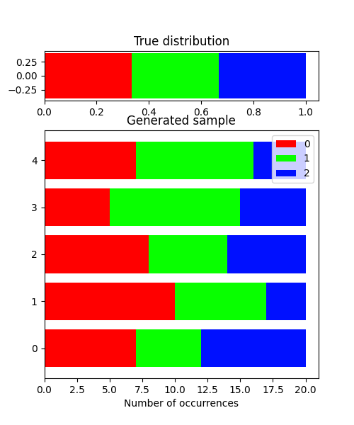
- visualize_model(sample_size=20, sample_num=5)#
Visualize the stochastic data generative model and generated samples.
- Parameters:
- sample_sizeint, optional
A positive integer, by default 20
- sample_numint, optional
A positive integer, by default 5
Examples
>>> from bayesml import categorical
>>> model = categorical.GenModel(3)
>>> model.visualize_model()
theta_vec:[0.33333333 0.33333333 0.33333333]
- class bayesml.categorical.LearnModel(c_degree, h0_alpha_vec=None)#
Bases:
Posterior,PredictiveMixinThe posterior distribution and the predictive distribution.
- Parameters:
- c_degreeint
a positive integer.
- h0_alpha_vecnumpy.ndarray, optional
a vector of positive real numbers, by default [1/2, 1/2, … , 1/2]. If a single real number is input, it will be broadcasted.
- Attributes:
- hn_alpha_vecnumpy.ndarray
a vector of positive real numbers
- p_theta_vecnumpy.ndarray
a real vector in \([0, 1]^d\)
Methods
Calculate log marginal likelihood
Calculate the parameters of the predictive distribution.
estimate_params([loss, dict_out])Estimate the parameter of the stochastic data generative model under the given criterion.
Get constants of LearnModel.
Get the initial values of the hyperparameters of the posterior distribution.
Get the hyperparameters of the posterior distribution.
Get the parameters of the predictive distribution.
load_h0_params(filename)Load the hyperparameters to h0_params.
load_hn_params(filename)Load the hyperparameters to hn_params.
make_prediction([loss, onehot])Predict a new data point under the given criterion.
overwrite_h0_params()Overwrite the initial values of the hyperparameters of the posterior distribution by the learned values.
pred_and_update(x[, loss, onehot])Predict a new data point and update the posterior sequentially.
reset_hn_params()Reset the hyperparameters of the posterior distribution to their initial values.
save_h0_params(filename)Save the hyperparameters using python
picklemodule.save_hn_params(filename)Save the hyperparameters using python
picklemodule.set_h0_params([h0_alpha_vec])Set the hyperparameters of the prior distribution.
set_hn_params([hn_alpha_vec])Set updated values of the hyperparameter of the posterior distribution.
update_posterior(x[, onehot])Update the hyperparameters of the posterior distribution using traning data.
Visualize the posterior distribution for the parameter.
- get_constants()#
Get constants of LearnModel.
- Returns:
- constantsdict of {str: int}
"c_degree": the value ofself.c_degree
- set_h0_params(h0_alpha_vec=None)#
Set the hyperparameters of the prior distribution.
- Parameters:
- h0_alpha_vecnumpy ndarray, optional
a vector of positive real numbers, by default None. If a single real number is input, it will be broadcasted.
- get_h0_params()#
Get the initial values of the hyperparameters of the posterior distribution.
- Returns:
- h0_paramsdict of {str: float, numpy.ndarray}
"h0_alpha_vec": The value ofself.h0_alpha_vec
- set_hn_params(hn_alpha_vec=None)#
Set updated values of the hyperparameter of the posterior distribution.
- Parameters:
- hn_alpha_vecnumpy ndarray, optional
a vector of positive real numbers, by default None. If a single real number is input, it will be broadcasted.
- get_hn_params()#
Get the hyperparameters of the posterior distribution.
- Returns:
- hn_paramsdict of {str: numpy.ndarray}
"hn_alpha_vec": The value ofself.hn_alpha_vec
- update_posterior(x, onehot=True)#
Update the hyperparameters of the posterior distribution using traning data.
- Parameters:
- xnumpy.ndarray
A non-negative int array. If onehot option is True, its shape must be
(sample_size,c_degree)and each row must be a one-hot vector. If onehot option is False, its shape must be(sample_size,)and each element must be smaller thanself.c_degree.- onehotbool, optional
If True, the input sample must be one-hot encoded, by default True.
- estimate_params(loss='squared', dict_out=False)#
Estimate the parameter of the stochastic data generative model under the given criterion.
- Parameters:
- lossstr, optional
Loss function underlying the Bayes risk function, by default “squared”. This function supports “squared”, “0-1”, and “KL”.
- dict_outbool, optional
If
True, output will be a dict, by defaultFalse.
- Returns:
- estimates{numpy ndarray, float, None, or rv_frozen}
The estimated values under the given loss function. If it is not exist, None will be returned. If the loss function is “KL”, the posterior distribution itself will be returned as rv_frozen object of scipy.stats.
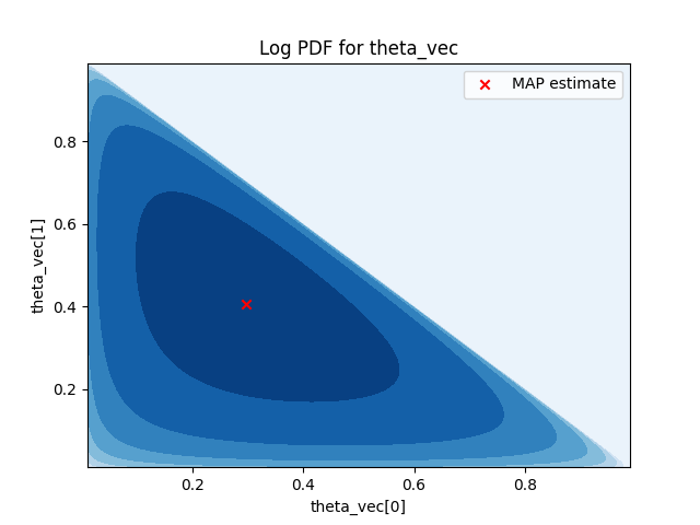
- visualize_posterior()#
Visualize the posterior distribution for the parameter.
Examples
>>> from bayesml import categorical
>>> gen_model = categorical.GenModel(3)
>>> x = gen_model.gen_sample(20)
>>> learn_model = categorical.LearnModel()
>>> learn_model.update_posterior(x)
>>> learn_model.visualize_posterior()
hn_alpha_vec:[6.5 8.5 6.5]
- get_p_params()#
Get the parameters of the predictive distribution.
- Returns:
- p_paramsdict of {str: numpy.ndarray}
"p_theta_vec": The value ofself.p_theta_vec
- calc_pred_dist()#
Calculate the parameters of the predictive distribution.
- make_prediction(loss='squared', onehot=True)#
Predict a new data point under the given criterion.
- Parameters:
- lossstr, optional
Loss function underlying the Bayes risk function, by default “squared”. This function supports “squared”, “0-1”, and “KL”.
- onehotbool, optional
If True, predected value under “0-1” loss will be one-hot encoded, by default True.
- Returns:
- Predicted_value{float, numpy.ndarray}
The predicted value under the given loss function. If the loss function is “KL”, the predictive distribution will be returned as 1-dimensional numpy.ndarray that consists of occurence probabilities.
- pred_and_update(x, loss='squared', onehot=True)#
Predict a new data point and update the posterior sequentially.
- Parameters:
- xnumpy.ndarray or int
If onehot option is True, 1-dimensional array whose length is
c_degree. If onehot option is False, a non-negative integer.- lossstr, optional
Loss function underlying the Bayes risk function, by default “squared”. This function supports “squared”, “0-1”, and “KL”.
- onehotbool, optional
If True, the input must be one-hot encoded and a predected value under “0-1” loss will be one-hot encoded, by default True.
- Returns:
- Predicted_value{int, numpy.ndarray}
The predicted value under the given loss function. If the loss function is “KL”, the predictive distribution itself will be returned as numpy.ndarray.
- calc_log_marginal_likelihood()#
Calculate log marginal likelihood
- Returns:
- log_marginal_likelihoodfloat
The log marginal likelihood.